Using flashlight

Overview

No black-box model without XAI. This is where packages like

{DALEX},
{iml}, and
{flashlight} enter the stage.

{flashlight} offers the following XAI methods:

light_performance(): Performance metrics like RMSE and/or $R^2$
light_importance(): Permutation variable importance (Fisher, Rudin, and Dominici 2018)
light_ice(): Individual conditional expectation (ICE) profiles (Goldstein et al. 2015) (centered or uncentered)
light_profile(): Partial dependence (Friedman 2001), accumulated local effects (ALE) (Apley and Zhu 2016), average predicted/observed/residual
light_profile2d(): Two-dimensional version of light_profile()
light_effects(): Combines partial dependence, ALE, response and prediction profiles
light_interaction(): Different variants of Friedman’s H statistics (Friedman and Popescu 2008)
light_breakdown(): Variable contribution breakdown (approximate SHAP) for single observations (Gosiewska and Biecek 2019)
light_global_surrogate(): Global surrogate trees (Molnar 2019)

Good to know:

Each method acts on an explainer object called flashlight (see examples and Section “flashlights”).
Multiple models can be compared via multiflashlight().
Calling plot() visualizes the results via {ggplot2}.
Methods support case weights.
Methods support a grouping variable.

Installation

# From CRAN
install.packages("flashlight")

# Development version
devtools::install_github("mayer79/flashlight")

Usage

Let’s start with an iris example. For simplicity, we do not split the data into training and testing/validation sets.

library(ggplot2)
library(MetricsWeighted)
library(flashlight)

fit_lm <- lm(Sepal.Length ~ ., data = iris)

# Make explainer object
fl_lm <- flashlight(
  model = fit_lm, 
  data = iris, 
  y = "Sepal.Length", 
  label = "lm",               
  metrics = list(RMSE = rmse, `R-squared` = r_squared)
)

Performance

fl_lm |> 
  light_performance() |> 
  plot(fill = "darkred") +
  labs(x = element_blank(), title = "Performance on training data")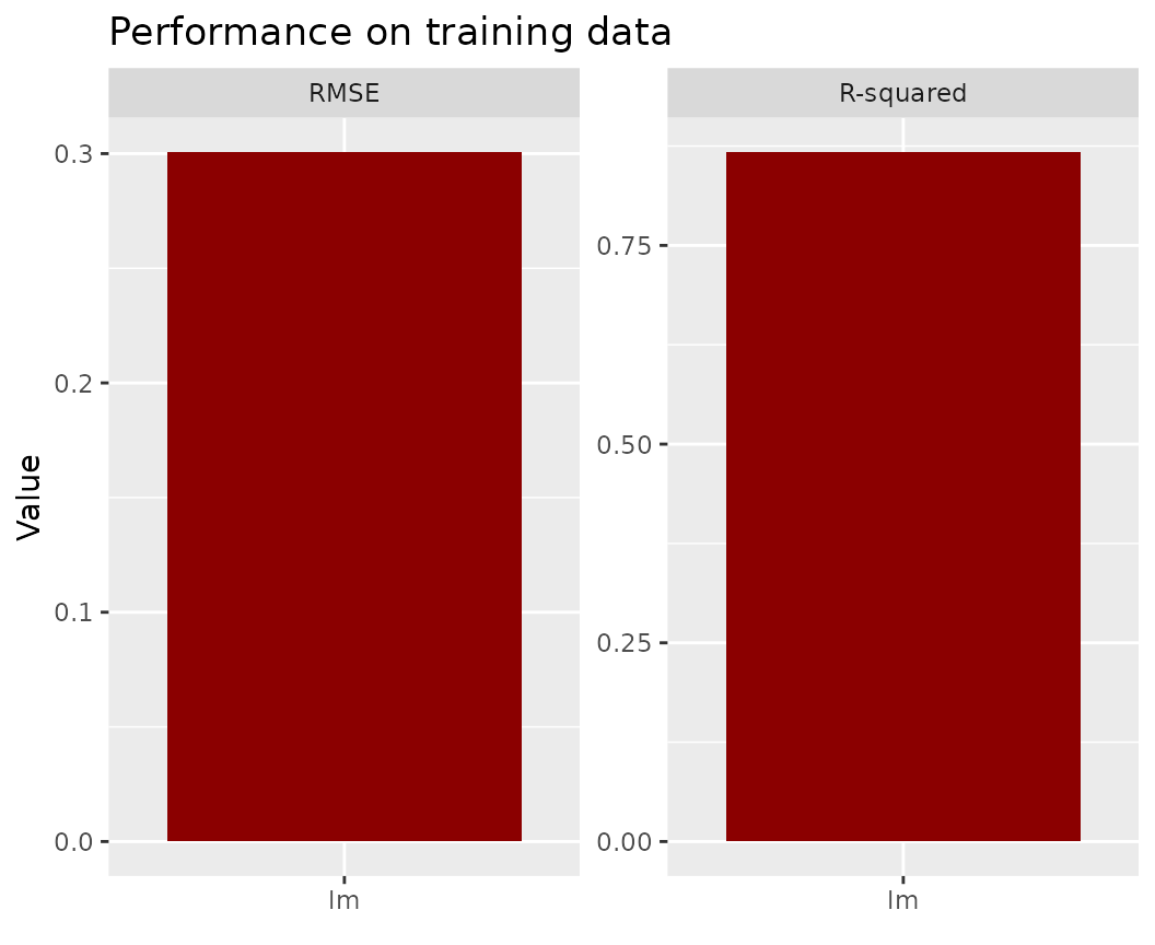


fl_lm |> 
  light_performance(by = "Species") |> 
  plot(fill = "darkred") +
  ggtitle("Performance split by Species")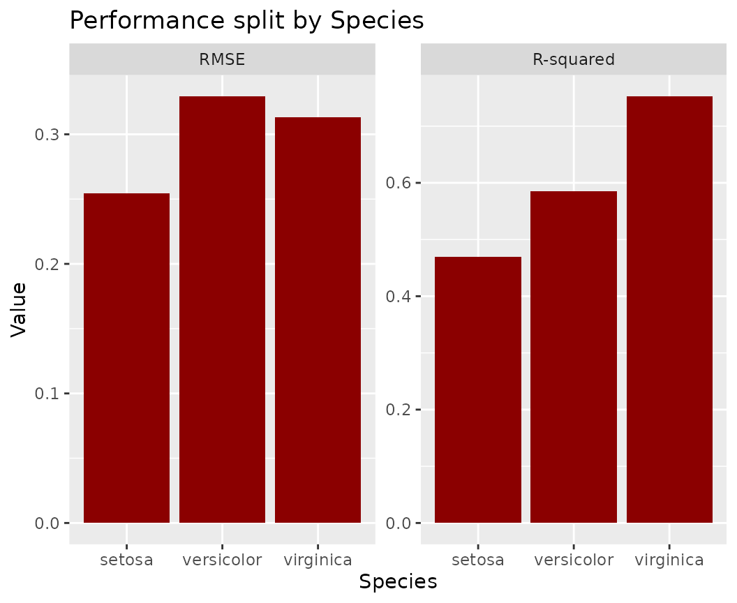

Permutation importance regarding first metric

Error bars represent standard errors, i.e., the uncertainty of the estimated importance.

fl_lm |>
  light_importance(m_repetitions = 4) |> 
  plot(fill = "darkred") +
  labs(title = "Permutation importance", y = "Increase in RMSE")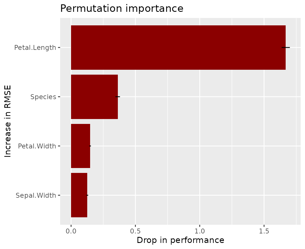

ICE curves for `Petal.Width`

fl_lm |> 
  light_ice("Sepal.Width", n_max = 200) |> 
  plot(alpha = 0.3, color = "chartreuse4") +
  labs(title = "ICE curves for 'Sepal.Width'", y = "Prediction")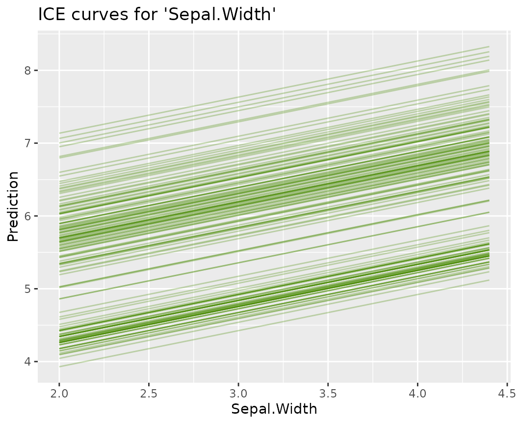


fl_lm |> 
  light_ice("Sepal.Width", n_max = 200, center = "middle") |> 
  plot(alpha = 0.3, color = "chartreuse4") +
  labs(title = "c-ICE curves for 'Sepal.Width'", y = "Prediction (centered)")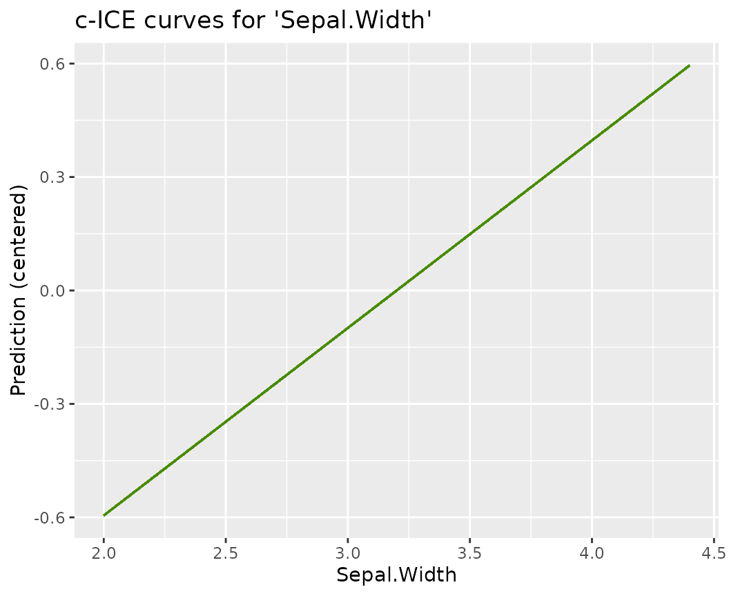

### PDPs

fl_lm |> 
  light_profile("Sepal.Width", n_bins = 40) |> 
  plot() +
  ggtitle("PDP for 'Sepal.Width'")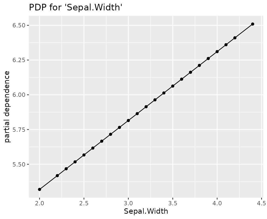


fl_lm |> 
  light_profile("Sepal.Width", n_bins = 40, by = "Species") |> 
  plot() +
  ggtitle("Same grouped by 'Species'")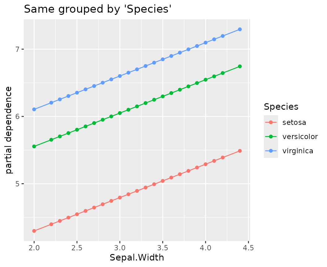

2D PDP

fl_lm |> 
  light_profile2d(c("Petal.Width", "Petal.Length")) |> 
  plot()

ALE

fl_lm |> 
  light_profile("Sepal.Width", type = "ale") |> 
  plot() +
  ggtitle("ALE plot for 'Sepal.Width'")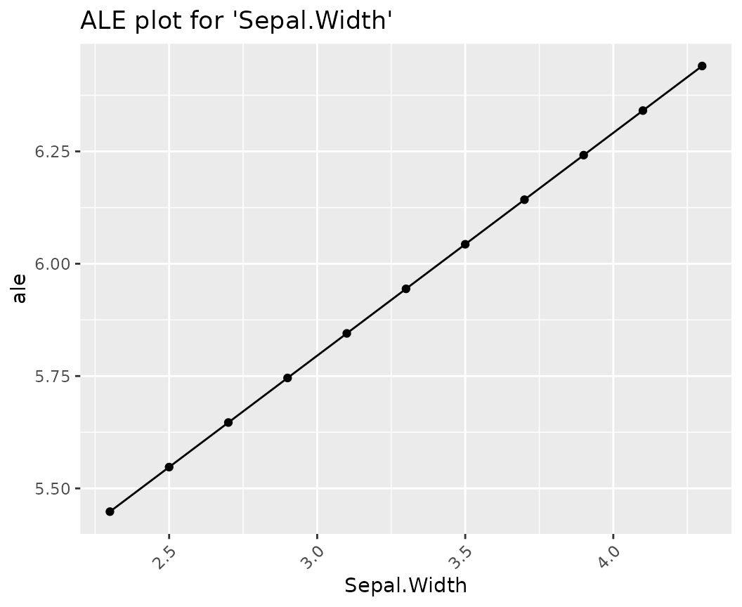

Different profile plots in one

fl_lm |> 
  light_effects("Sepal.Width") |> 
  plot(use = "all") +
  ggtitle("Different types of profiles for 'Sepal.Width'")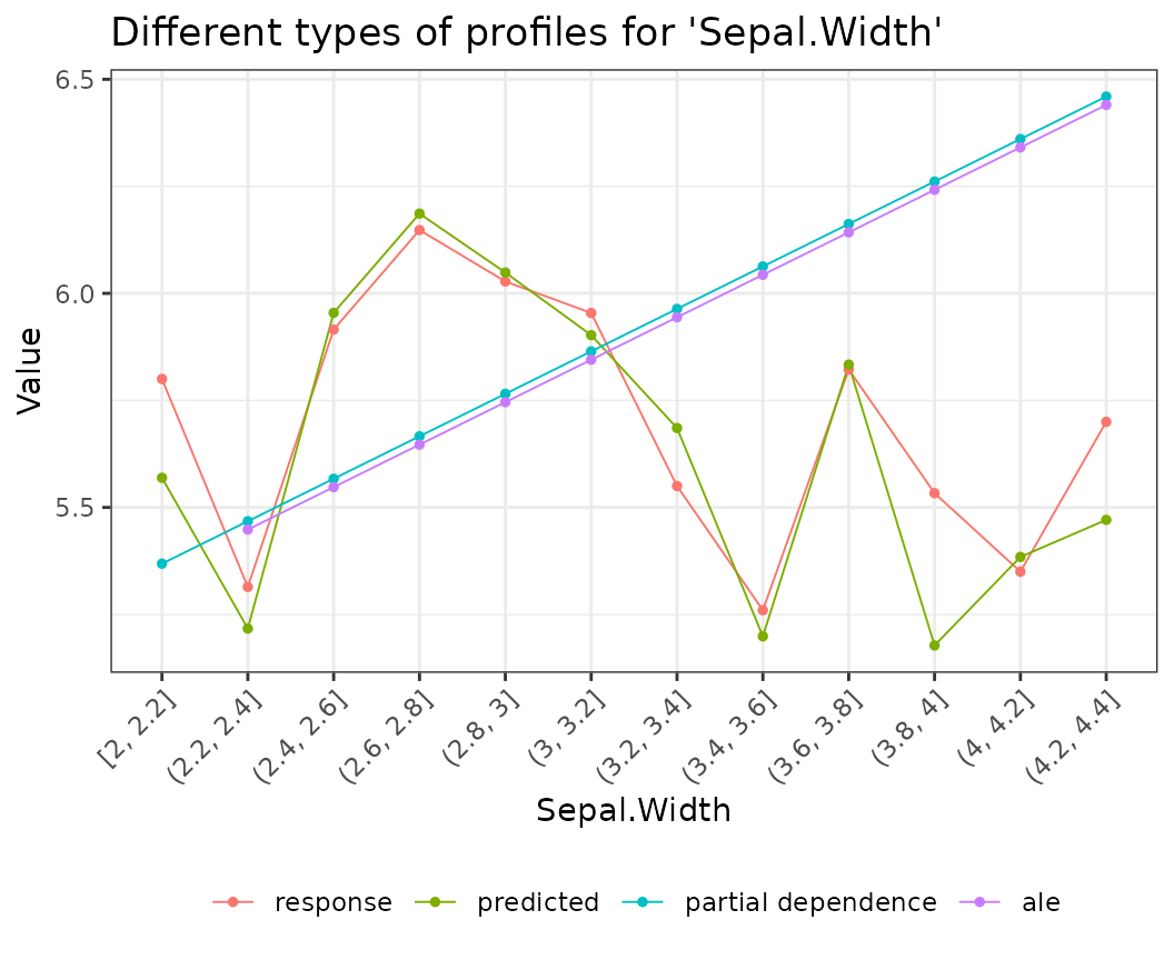

Variable contribution breakdown for single observation

fl_lm |> 
  light_breakdown(new_obs = iris[1, ]) |> 
  plot()

Global surrogate tree

fl_lm |> 
  light_global_surrogate() |> 
  plot()

### Multiple models

Multiple flashlights can be combined to a multiflashlight.

library(rpart)

fit_tree <- rpart(
  Sepal.Length ~ ., 
  data = iris, 
  control = list(cp = 0, xval = 0, maxdepth = 5)
)

# Make explainer object
fl_tree <- flashlight(
  model = fit_tree, 
  data = iris, 
  y = "Sepal.Length", 
  label = "tree",               
  metrics = list(RMSE = rmse, `R-squared` = r_squared)
)

# Combine with other explainer
fls <- multiflashlight(list(fl_tree, fl_lm))

fls |> 
  light_performance() |> 
  plot(fill = "chartreuse4") +
  labs(x = "Model", title = "Performance")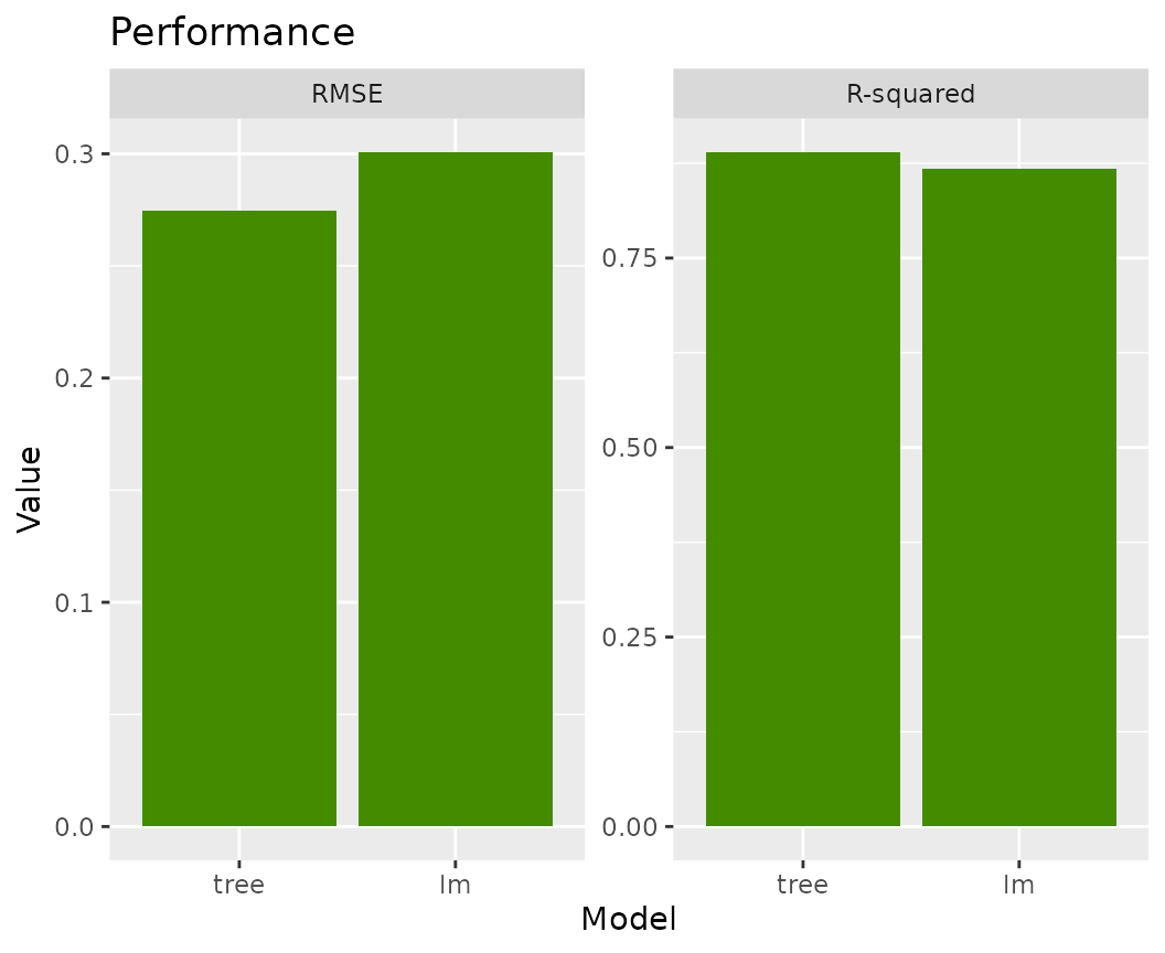


fls |> 
  light_importance() |> 
  plot(fill = "chartreuse4") +
  labs(y = "Increase in RMSE", title = "Permutation importance")


fls |> 
  light_profile("Petal.Length", n_bins = 40) |> 
  plot() +
  ggtitle("PDP")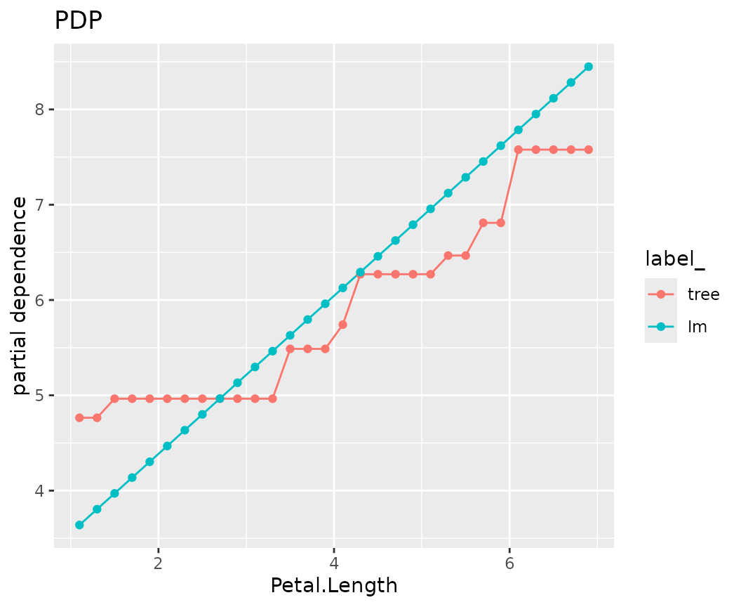


fls |> 
  light_profile("Petal.Length", n_bins = 40, by = "Species") |> 
  plot() +
  ggtitle("PDP by Species")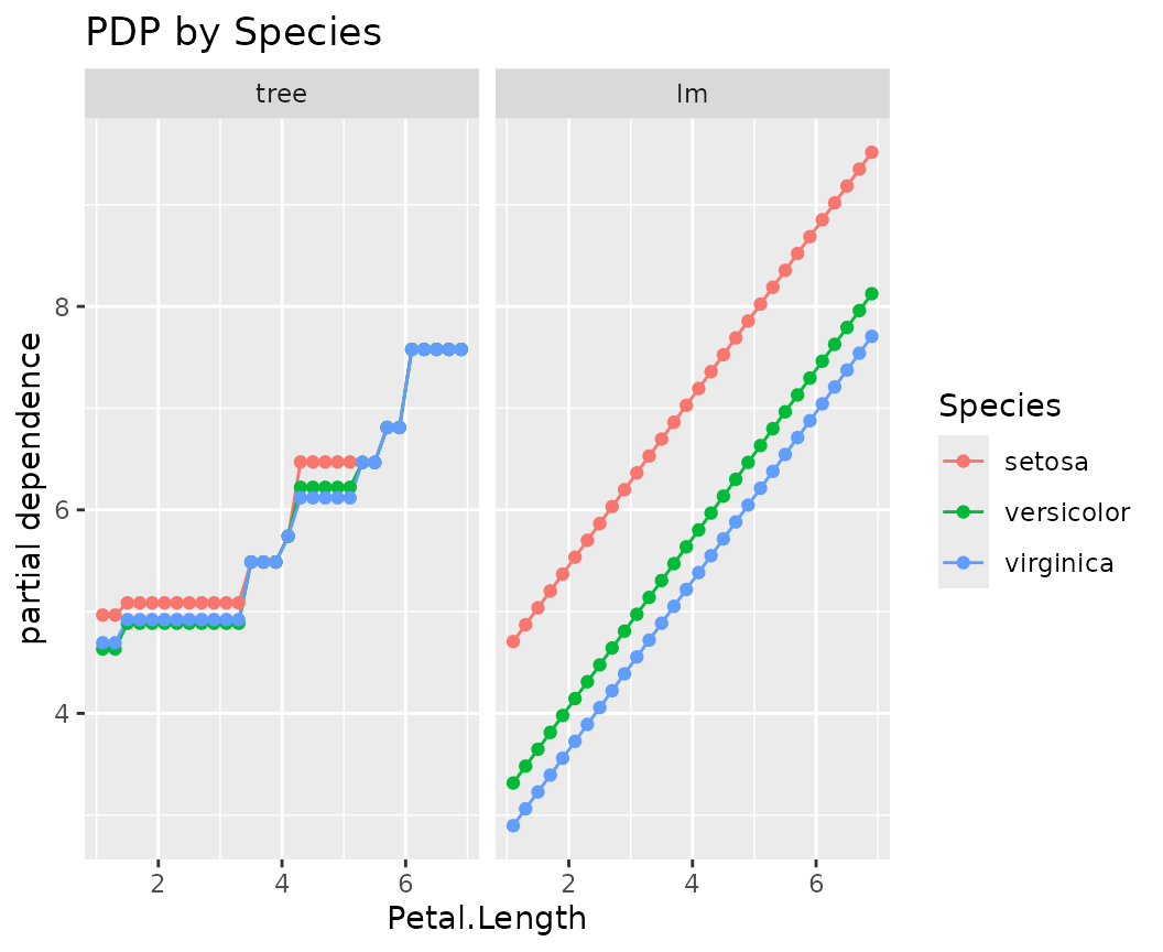

flashlights

The “flashlight” explainer expects the following information:

model: Fitted model. Currently, this argument must be named.
data: Reference data used to calculate things, often part of the validation data.
y: Column name in data corresponding to the numeric response.
predict_function: function of the same signature as stats::predict(). It takes a model and a data.frame data, and provides numeric predictions, see below for more details.
linkinv: Optional function applied to the output of predict_function(). Should actually be called “trafo”.
w: Optional column name in data corresponding to case weights.
by: Optional column name in data used to group the results. Must be discrete.
metrics: List of metrics, by default list(rmse = MetricsWeighted::rmse). For binary (probabilistic) classification, good candidate metrics would be MetricsWeighted::logLoss.
label: Mandatory name of the model.

Typical `predict_function`s (a selection)

The default stats::predict() works for models of class

lm(),
glm() (for predictions on link scale), and
rpart().

It also works for meta-learner models like

{caret}, and
{mlr3}.

Manual prediction functions are, e.g., required for

{ranger}: Use function(m, X) predict(m, X)$predictions for regression, and function(m, X) predict(m, X)$predictions[, 2] for probabilistic binary classification
glm(): Use function(m, X) predict(m, X, type = "response") to get GLM predictions at the response scale

A bit more complicated are models whose native predict function do not work on data.frames:

{xgboost} and {lightgbm}: They digest numeric matrices only, so the prediction function also needs to deal with the mapping from data.frame to matrix.
{keras}: It might accept data.frame inputs, but we need to take care of scalings.

Example (XGBoost):

This works when non-numeric features are all factors (not categoricals):

x <- vector of features
predict_function = function(m, df) predict(m, data.matrix(df[x]))

References

Apley, Daniel W., and Jingyu Zhu. 2016. “Visualizing the Effects of Predictor Variables in Black Box Supervised Learning Models.” https://arxiv.org/abs/1612.08468.

Fisher, Aaron, Cynthia Rudin, and Francesca Dominici. 2018. “All Models Are Wrong, but Many Are Useful: Learning a Variable’s Importance by Studying an Entire Class of Prediction Models Simultaneously.” https://arxiv.org/abs/1801.01489.

Friedman, Jerome H. 2001. “Greedy Function Approximation: A Gradient Boosting Machine.” Ann. Statist. 29 (5): 1189–1232. https://doi.org/10.1214/aos/1013203451.

Friedman, Jerome H., and Bogdan E. Popescu. 2008. “Predictive Learning via Rule Ensembles.” The Annals of Applied Statistics 2 (3): 916–54.

Goldstein, Alex, Adam Kapelner, Justin Bleich, and Emil Pitkin. 2015. “Peeking Inside the Black Box: Visualizing Statistical Learning with Plots of Individual Conditional Expectation.” Journal of Computational and Graphical Statistics 24 (1): 44–65. https://doi.org/10.1080/10618600.2014.907095.

Gosiewska, Alicja, and Przemyslaw Biecek. 2019. “Do Not Trust Additive Explanations.” https://arxiv.org/abs/1903.11420.

Molnar, Christoph. 2019. Interpretable Machine Learning: A Guide for Making Black Box Models Explainable. https://christophm.github.io/interpretable-ml-book/.