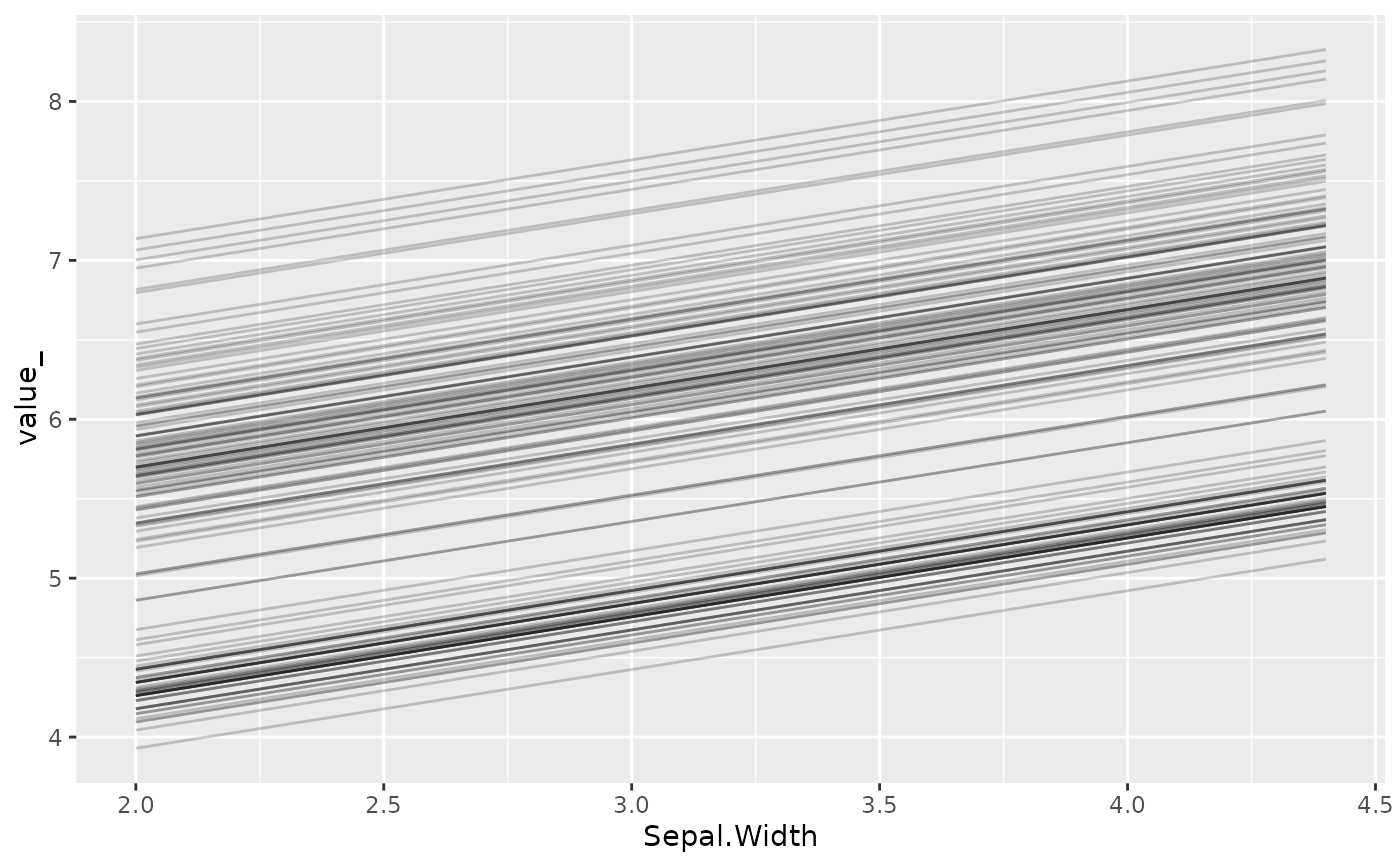
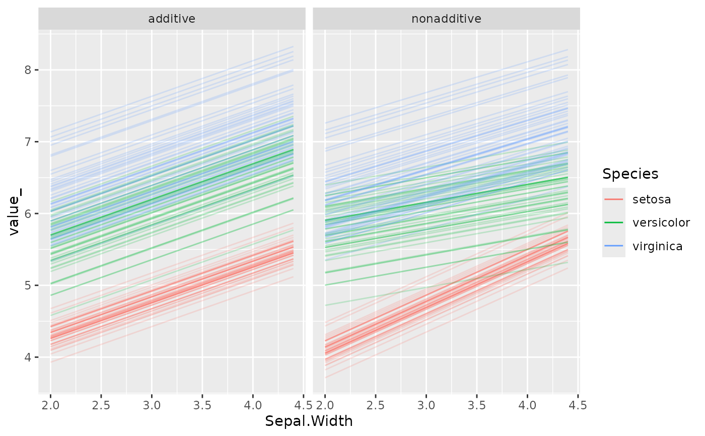
Generates Individual Conditional Expectation (ICE) profiles. An ICE profile shows how the prediction of an observation changes if one or multiple variables are systematically changed across its ranges, holding all other values fixed (see the reference below for details). The curves can be centered in order to increase visibility of interaction effects.
light_ice(x, ...)

# Default S3 method
light_ice(x, ...)

# S3 method for class 'flashlight'
light_ice(
  x,
  v = NULL,
  data = x$data,
  by = x$by,
  evaluate_at = NULL,
  breaks = NULL,
  grid = NULL,
  n_bins = 27L,
  cut_type = c("equal", "quantile"),
  indices = NULL,
  n_max = 20L,
  seed = NULL,
  use_linkinv = TRUE,
  center = c("no", "first", "middle", "last", "mean", "0"),
  ...
)

# S3 method for class 'multiflashlight'
light_ice(x, ...)
Arguments
- x
An object of class "flashlight" or "multiflashlight".
- ...
Further arguments passed to or from other methods.
- v
The variable name to be profiled.
- data
An optional
data.frame.- by
An optional vector of column names used to additionally group the results.
- evaluate_at
Vector with values of
vused to evaluate the profile.- breaks
Cut breaks for a numeric
v. Used to overwrite automatic binning vian_binsandcut_type. Ignored ifvis not numeric or ifgridorevaluate_atare specified.- grid
A
data.framewith evaluation grid. For instance, can be generated byexpand.grid().- n_bins
Approximate number of unique values to evaluate for numeric
v. Ignored ifvis not numeric or ifbreaks,gridorevaluate_atare specified.- cut_type
Should a numeric
vbe cut into "equal" or "quantile" bins? Ignored ifvis not numeric or ifbreaks,gridorevaluate_atare specified.- indices
A vector of row numbers to consider.
- n_max
If
indicesis not given, maximum number of rows to consider. Will be randomly picked fromdataif necessary.- seed
An integer random seed.
- use_linkinv
Should retransformation function be applied? Default is
TRUE.- center
How should curves be centered?
Default is "no".
Choose "first", "middle", or "last" to 0-center at specific evaluation points.
Choose "mean" to center all profiles at the within-group means.
Choose "0" to mean-center curves at 0.
Value
An object of class "light_ice" with the following elements:
dataA tibble containing the results.bySame as inputby.vThe variable(s) evaluated.centerHow centering was done.
Details
There are two ways to specify the variable(s) to be profiled.
Pass the variable name via
vand an optional vector with evaluation pointsevaluate_at(orbreaks). This works for dependence on a single variable.More general: Specify any
gridas adata.framewith one or more columns. For instance, it can be generated by a call toexpand.grid().
The minimum required elements in the (multi-)flashlight are "predict_function", "model", "linkinv" and "data", where the latest can be passed on the fly.
Which rows in data are profiled? This is specified by indices.
If not given and n_max is smaller than the number of rows in data,
then row indices will be sampled randomly from data.
If the same rows should be used for all flashlights in a multiflashlight,
there are two options: Either pass a seed or a vector of indices used to select rows.
In both cases, data should be the same for all flashlights considered.
Methods (by class)
light_ice(default): Default method not implemented yet.light_ice(flashlight): ICE profiles for a flashlight object.light_ice(multiflashlight): ICE profiles for a multiflashlight object.
References
Goldstein, A. et al. (2015). Peeking inside the black box: Visualizing statistical learning with plots of individual conditional expectation. Journal of Computational and Graphical Statistics, 24:1 <doi.org/10.1080/10618600.2014.907095>.
See also
Examples
fit_add <- lm(Sepal.Length ~ ., data = iris)
fl_add <- flashlight(model = fit_add, label = "additive", data = iris)

plot(light_ice(fl_add, v = "Sepal.Width", n_max = 200), alpha = 0.2)

plot(light_ice(fl_add, v = "Sepal.Width", n_max = 200, center = "first"))


# Second model with interactions
fit_nonadd <- lm(Sepal.Length ~ . + Sepal.Width:Species, data = iris)
fl_nonadd <- flashlight(model = fit_nonadd, label = "nonadditive", data = iris)
fls <- multiflashlight(list(fl_add, fl_nonadd))

plot(light_ice(fls, v = "Sepal.Width", by = "Species", n_max = 200), alpha = 0.2)

plot(light_ice(fls, v = "Sepal.Width", by = "Species", n_max = 200, center = "mid"))
