Overview
{outForest} is a random forest-based implementation of the method described in Chapter 7.1.2 (“Regression model based anomaly detection”) of (Chandola, Banerjee, and Kumar 2009). Each numeric variable is regressed onto all other variables using a random forest. If the scaled absolute difference between observed value and out-of-bag prediction is suspiciously large (e.g., more than three times the RMSE of the out-of-bag predictions), then a value is considered an outlier. After identification of outliers, they can be replaced, for instance, by predictive mean matching from the non-outliers.
The method can be viewed as a multivariate extension of a basic univariate outlier detection method, in which a value is considered an outlier if it deviates from the mean by more than, say, three times the standard deviation. In the multivariate case, instead of comparing a value with the overall mean, rather the difference to the conditional mean is considered. {outForest} estimates this conditional mean by a random forest.
Specifically, the outlier score of the -th observed value of variable is defined as where is the corresponding out-of-bag prediction of the -th random forest with RMSE . If with threshold , then is considered an outlier.
Why using random forests for calculating the conditional means? They often work well without parameter tuning, outliers in the input variables are no issue and the out-of-bag mechanism helps to provide fair outlier scores.
{outForest} utilizes the high-performance random forest implementation {ranger} (Wright and Ziegler 2017). Since it does not allow for missing values, any missing value is first being imputed by chained random forests implemented in {missRanger}.
In the examples below, we will meet different functions from the {outForest} package:
outForest(): This is the main function. It identifies and replaces outliers in numeric variables of a data frame.print(),summary()andplot(): To inspect outlier information.outliers()andData(): To extract information on outliers and the data with replaced outliers.generateOutliers(): To add nasty outliers to a data set.predict(): To apply a fitted “outForest” object to fresh data.
Installation
# From CRAN
install.packages("outForest")

# Development version
devtools::install_github("mayer79/outForest")
Usage
We first generate a data set with two multivariate outliers. Then, we
use outForest() to find them.
library(outForest)

# Create data with multivariate outlier
set.seed(3)
t <- seq(0, pi, by = 0.01)
dat <- data.frame(x = cos(t), y = sin(t) + runif(length(t), -0.1, 0.1))
dat[c(100, 200), ] <- cbind(c(-0.5, 0.5), c(0.4, 0.4))

plot(y ~ x, data = dat)
# Let's run outForest on that data
ch <- outForest(dat)
#>
#> Outlier identification by random forests
#>
#>   Variables to check:        x, y
#>   Variables used to check:   x, y
#>
#>   Checking: x  y

# What outliers did we find?
outliers(ch)
#>   row col observed predicted       rmse     score threshold replacement
#> 1 100   y      0.4 0.8567112 0.07485516 -6.101265         3   0.9913182
#> 2 200   y      0.4 0.8244413 0.07485516 -5.670168         3   0.8113720

# Bingo! How does the fixed data set looks like?
plot(y ~ x, data = Data(ch))
# The number of outliers per variable
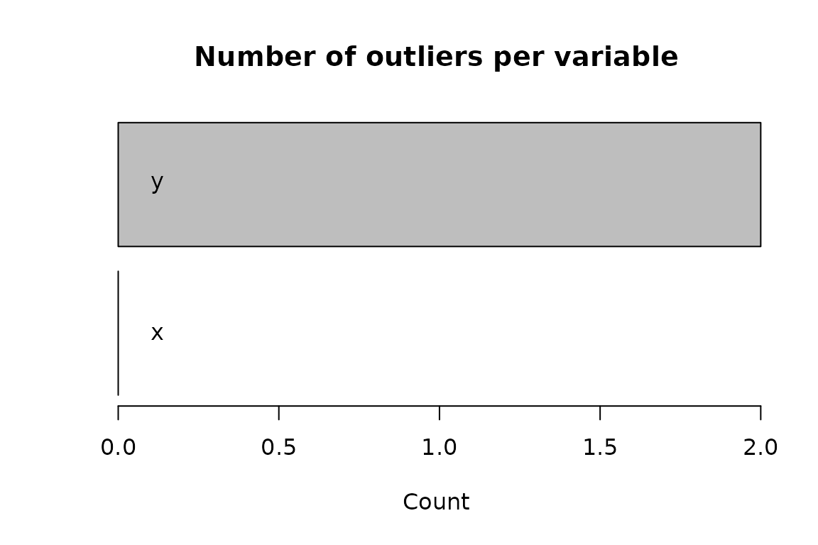
plot(ch)
Note that outForest() offers a ... argument
to pass options to its workhorse random forest implementation
ranger(), e.g., num.trees or
mtry. How would we use its “extra trees” variant with 50
trees? As data set, we add a couple of outliers to the famous iris
flower data set.
head(irisWithOutliers <- generateOutliers(iris, p = 0.02))
#>   Sepal.Length Sepal.Width Petal.Length Petal.Width Species
#> 1          5.1         3.5      1.40000         0.2  setosa
#> 2          4.9         3.0    -13.32449         0.2  setosa
#> 3          4.7         3.2      1.30000         0.2  setosa
#> 4          4.6         3.1      1.50000         0.2  setosa
#> 5          5.0         3.6      1.40000         0.2  setosa
#> 6          5.4         3.9      1.70000         0.4  setosa
out <- outForest(
  irisWithOutliers, splitrule = "extratrees", num.trees = 50, verbose = 0
)

# The worst outliers
head(outliers(out))
#>   row          col   observed predicted      rmse     score threshold
#> 9  77  Petal.Width   8.617485  1.462865 0.6365155 11.240290         3
#> 7   2 Petal.Length -13.324488  1.572715 1.5200990 -9.800153         3
#> 6 135  Sepal.Width  -5.061389  3.120949 0.9375457 -8.727402         3
#> 1  66 Sepal.Length  16.880345  6.070454 1.4580339  7.414019         3
#> 2 127 Sepal.Length  -4.004644  6.355322 1.4580339 -7.105436         3
#> 8 136 Petal.Length  -4.054545  5.790103 1.5200990 -6.476321         3
#>   replacement
#> 9         1.5
#> 7         1.3
#> 6         3.0
#> 1         6.1
#> 2         7.3
#> 8         6.7

# Summary of outliers
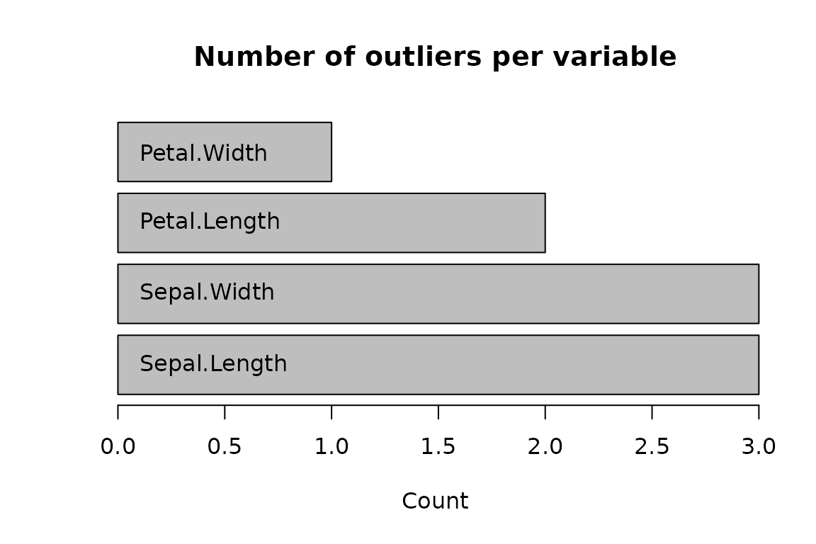
summary(out)
#> The following outlier counts have been detected:
#>
#>              Number of outliers
#> Sepal.Length                  3
#> Sepal.Width                   3
#> Petal.Length                  2
#> Petal.Width                   1
#>
#> These are the worst outliers:
#>
#>   row          col   observed predicted      rmse     score threshold
#> 9  77  Petal.Width   8.617485  1.462865 0.6365155 11.240290         3
#> 7   2 Petal.Length -13.324488  1.572715 1.5200990 -9.800153         3
#> 6 135  Sepal.Width  -5.061389  3.120949 0.9375457 -8.727402         3
#> 1  66 Sepal.Length  16.880345  6.070454 1.4580339  7.414019         3
#> 2 127 Sepal.Length  -4.004644  6.355322 1.4580339 -7.105436         3
#> 8 136 Petal.Length  -4.054545  5.790103 1.5200990 -6.476321         3
#>   replacement
#> 9         1.5
#> 7         1.3
#> 6         3.0
#> 1         6.1
#> 2         7.3
#> 8         6.7

# Basic plot of the number of outliers per variable
plot(out)
# Basic plot of the scores of the outliers per variable
plot(out, what = "scores")
Pipe
outForest() can be combined with the pipe:
Out-of-sample application
Once an “outForest” object is fitted with option
allow_predictions = TRUE, it can be used to find and
replace outliers in new data without refitting. Note that random forests
can be huge, so use this option with care. Further note that currently,
missing values in the new data are only allowed in one single variable
to be checked.
out <- outForest(iris, allow_predictions = TRUE, verbose = 0)
iris1 <- iris[1:2, ]
iris1$Sepal.Length[1] <- -1
pred <- predict(out, newdata = iris1)
outliers(pred)
#>   row          col observed predicted     rmse     score threshold replacement
#> 1   1 Sepal.Length       -1  5.011421 0.369207 -16.28198         3         5.2
Data(pred)
#>   Sepal.Length Sepal.Width Petal.Length Petal.Width Species
#> 1          5.2         3.5          1.4         0.2  setosa
#> 2          4.9         3.0          1.4         0.2  setosa
The formula interface
By default, outForest() uses all columns in the data set
to check all numeric columns with missings. To override this behavior,
you can use its formula interface: The left hand side specifies the
variables to be checked (variable names separated by a +),
while the right hand side lists the variables used for checking.
If you want to check only variable Sepal.Length based on
Species, then use this syntax.
out <- outForest(irisWithOutliers, Sepal.Length ~ Species, verbose = 0)
summary(out)
#> The following outlier counts have been detected:
#>
#>              Number of outliers
#> Sepal.Length                  3
#>
#> These are the worst outliers:
#>
#>   row          col  observed predicted     rmse     score threshold replacement
#> 1  66 Sepal.Length 16.880345  5.928826 1.490069  7.349674         3         5.9
#> 2 127 Sepal.Length -4.004644  6.752837 1.490069 -7.219453         3         6.4
#> 3 135 Sepal.Length 13.663652  6.381728 1.490069  4.886972         3         7.4
If you want to prevent outForest() to identify and
replace outliers in the response variable of a subsequent model,
Sepal.Length say, subtract that variable from the left hand
side.
out <- outForest(irisWithOutliers, . - Sepal.Length ~ ., verbose = 0)
summary(out)
#> The following outlier counts have been detected:
#>
#>              Number of outliers
#> Sepal.Width                   4
#> Petal.Length                  2
#> Petal.Width                   1
#>
#> These are the worst outliers:
#>
#>   row          col   observed  predicted      rmse     score threshold
#> 7  77  Petal.Width   8.617485  1.5489019 0.6485071 10.899777         3
#> 5   2 Petal.Length -13.324488  1.4629804 1.5531209 -9.521131         3
#> 4 135  Sepal.Width  -5.061389  3.2467161 0.9712182 -8.554314         3
#> 6 136 Petal.Length  -4.054545  6.0022195 1.5531209 -6.475198         3
#> 3 117  Sepal.Width   8.720982  2.9949163 0.9712182  5.895756         3
#> 2  66  Sepal.Width   3.100000 -0.8153869 0.9712182  4.031418         3
#>   replacement
#> 7         1.5
#> 5         1.4
#> 4         2.8
#> 6         5.9
#> 3         2.9
#> 2         2.4
Too many values are identified as outliers. Crap!
For large data sets, just by chance, many values can surpass the
default threshold of 3. To reduce the number of outliers, the threshold
can be increased. Alternatively, the number of outliers can be limited
by the two arguments max_n_outliers and
max_prop_outliers. For instance, if at most three outliers
are to be identified, set max_n_outliers = 3. If at most 1%
of the values are to be declared as outliers, set
max_prop_outliers = 0.01.
outliers(outForest(irisWithOutliers, max_n_outliers = 3, verbose = 0))
#>   row          col   observed predicted      rmse     score threshold
#> 3  77  Petal.Width   8.617485  1.575285 0.6447998 10.921528  7.501523
#> 2   2 Petal.Length -13.324488  1.451632 1.5567481 -9.491657  7.501523
#> 1 135  Sepal.Width  -5.061389  3.219084 0.9663933 -8.568430  7.501523
#>   replacement
#> 3         1.5
#> 2         1.4
#> 1         3.1
I don’t want outliers to be replaced!
By default outForest() replaces outliers by predictive
mean matching on the out-of-bag predictions. Alternatively, you can set
the replace argument to a different value:
"no": Outliers are not replaced."predicted": Outliers are replaced by the out-of-bag predictions (without predictive mean matching)."NA": Outliers are replaced by missing values.
So if you would like to replace outliers by NAs, write:
out <- outForest(irisWithOutliers, replace = "NA", verbose = 0)
head(Data(out))
#>   Sepal.Length Sepal.Width Petal.Length Petal.Width Species
#> 1          5.1         3.5          1.4         0.2  setosa
#> 2          4.9         3.0           NA         0.2  setosa
#> 3          4.7         3.2          1.3         0.2  setosa
#> 4          4.6         3.1          1.5         0.2  setosa
#> 5          5.0         3.6          1.4         0.2  setosa
#> 6          5.4         3.9          1.7         0.4  setosa
The algorithm takes too much time. What can I do?
By default, outForest() fits a random forest with 500
trees per numeric variable. Thus, the overall process can take very
long. Here a few tweaks to make things faster:
- Use less trees, e.g., by setting
num.trees = 50. - Use smaller mtry, e.g.,
mtry = 2. - Use shorter trees, e.g., setting
max.depth = 6. - Use large leaves, e.g.,
min.node.size = 10000.