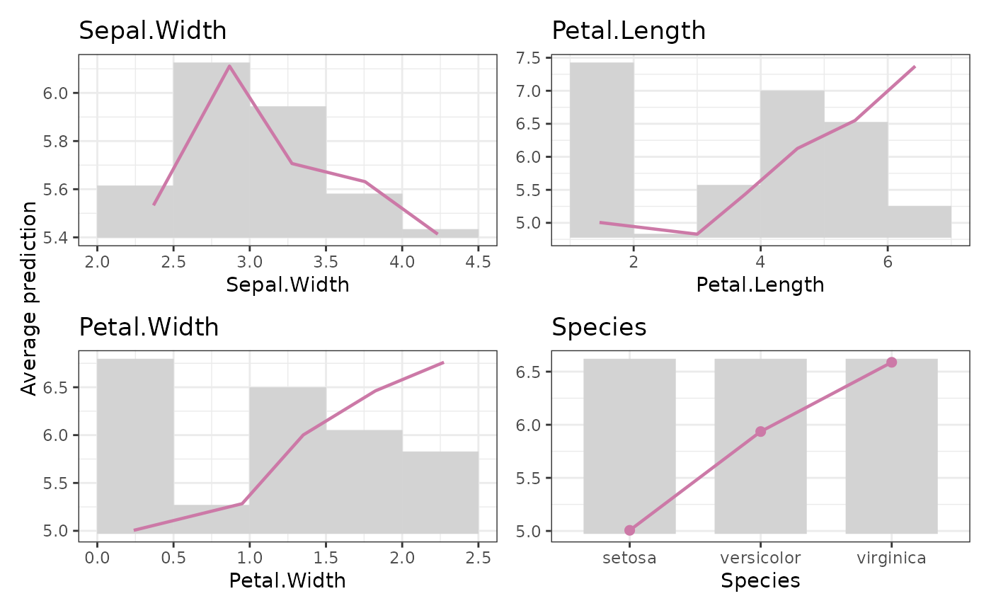
Calculates average predictions over the values of one or multiple features specified
by X. Shows the combined effect of a feature and other (correlated) features.
average_predicted(
  X,
  pred,
  w = NULL,
  x_name = "x",
  breaks = "Sturges",
  right = TRUE,
  discrete_m = 13L,
  outlier_iqr = 2,
  seed = NULL,
  ...
)
Arguments
- X
A vector, matrix, or data.frame with features.
- pred
A numeric vector of predictions.
- w
An optional numeric vector of weights. Having observations with non-positive weight is equivalent to excluding them.
- x_name
If
Xis a vector: what is the name of the variable? By default "x".- breaks
An integer, vector, or "Sturges" (the default) used to determine bin breaks of continuous features. Values outside the total bin range are placed in the outmost bins. To allow varying values of
breaksacross features,breakscan be a list of the same length asv, or a named list with breaks for certain variables.- right
Should bins be right-closed? The default is
TRUE. Vectorized overv. Only relevant for continuous features.- discrete_m
Numeric features with up to this number of unique values should not be binned but rather treated as discrete. The default is 13. Vectorized over
v.- outlier_iqr
If
breaksis an integer or "Sturges", the breaks of a continuous feature are calculated without taking into account feature values outside quartiles +-outlier_iqr* IQR (where <= 9997 values are used to calculate the quartiles). To let the breaks cover the full data range, setoutlier_iqrto 0 orInf. Vectorized overv.- seed
Optional integer random seed used for calculating breaks: The bin range is determined without values outside quartiles +- 2 IQR using a sample of <= 9997 observations to calculate quartiles.
- ...
Currently unused.
Value
A list (of class "EffectData") with a data.frame per feature having columns:
bin_mid: Bin mid points. In the plots, the bars are centered around these.bin_width: Absolute width of the bin. In the plots, these equal the bar widths.bin_mean: For continuous features, the (possibly weighted) average feature value within bin. For discrete features equivalent tobin_mid.N: The number of observations within bin.weight: The weight sum within bin. Whenw = NULL, equivalent toN.Different statistics, depending on the function call.
Use single bracket subsetting to select part of the output. Note that each data.frame contains an attribute "discrete" with the information whether the feature is discrete or continuous. This attribute might be lost when you manually modify the data.frames.
Details
The function is a convenience wrapper around feature_effects().
References
Apley, Daniel W., and Jingyu Zhu. 2016. Visualizing the Effects of Predictor Variables in Black Box Supervised Learning Models. Journal of the Royal Statistical Society Series B: Statistical Methodology, 82 (4): 1059–1086. doi:10.1111/rssb.12377.
See also
Examples
fit <- lm(Sepal.Length ~ ., data = iris)
M <- average_predicted(iris[2:5], pred = predict(fit, iris), breaks = 5)
M
#> 'EffectData' object of length 4, starting with 'Sepal.Width':
#>
#>   bin_mid bin_width bin_mean  N weight pred_mean
#> 1    2.25       0.5 2.368421 19     19  5.532860
#> 2    2.75       0.5 2.867188 64     64  6.111200
#> 3    3.25       0.5 3.277083 48     48  5.706627
#> 4    3.75       0.5 3.756250 16     16  5.631317
#> 5    4.25       0.5 4.233333  3      3  5.413218
M |> plot()
