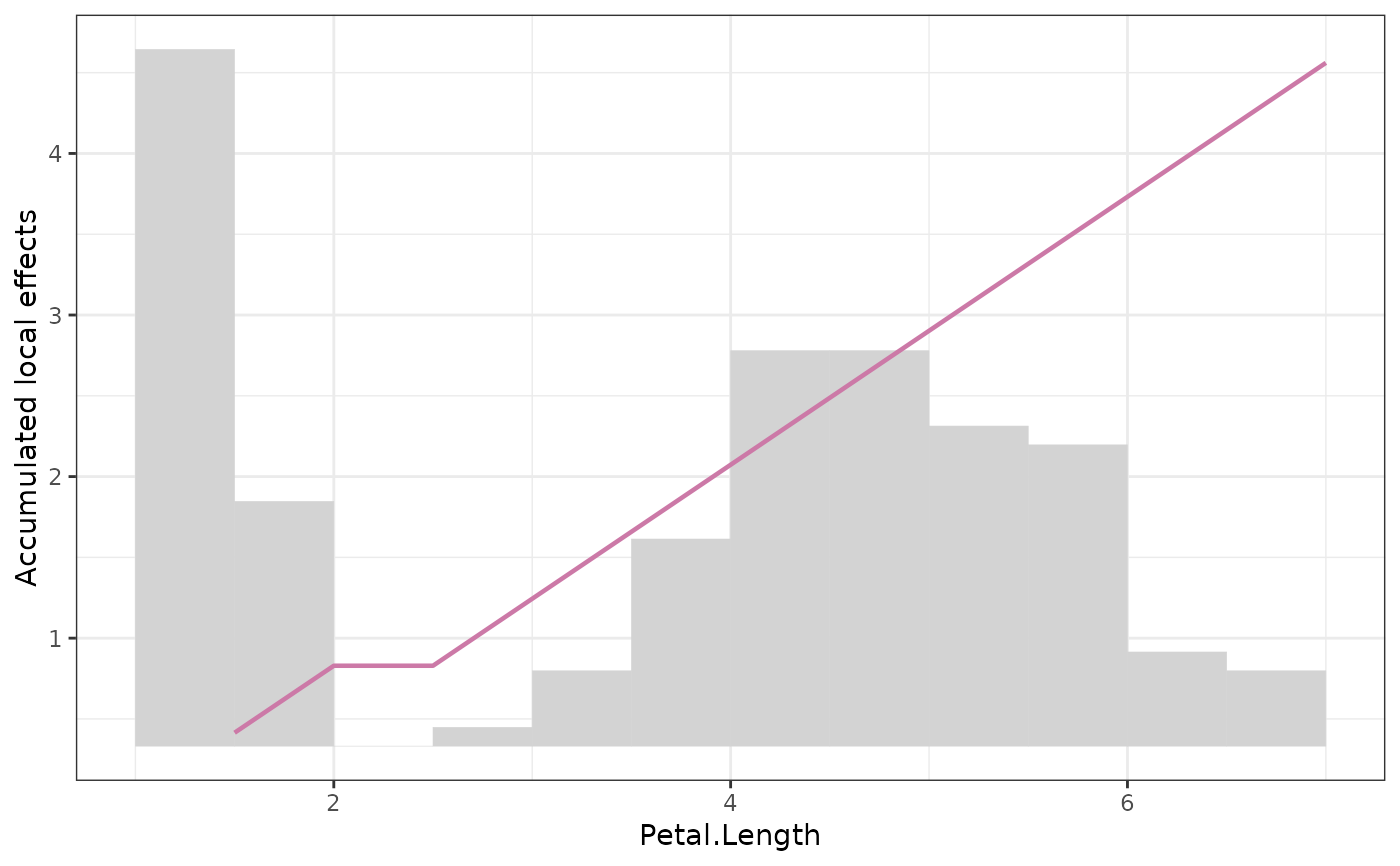
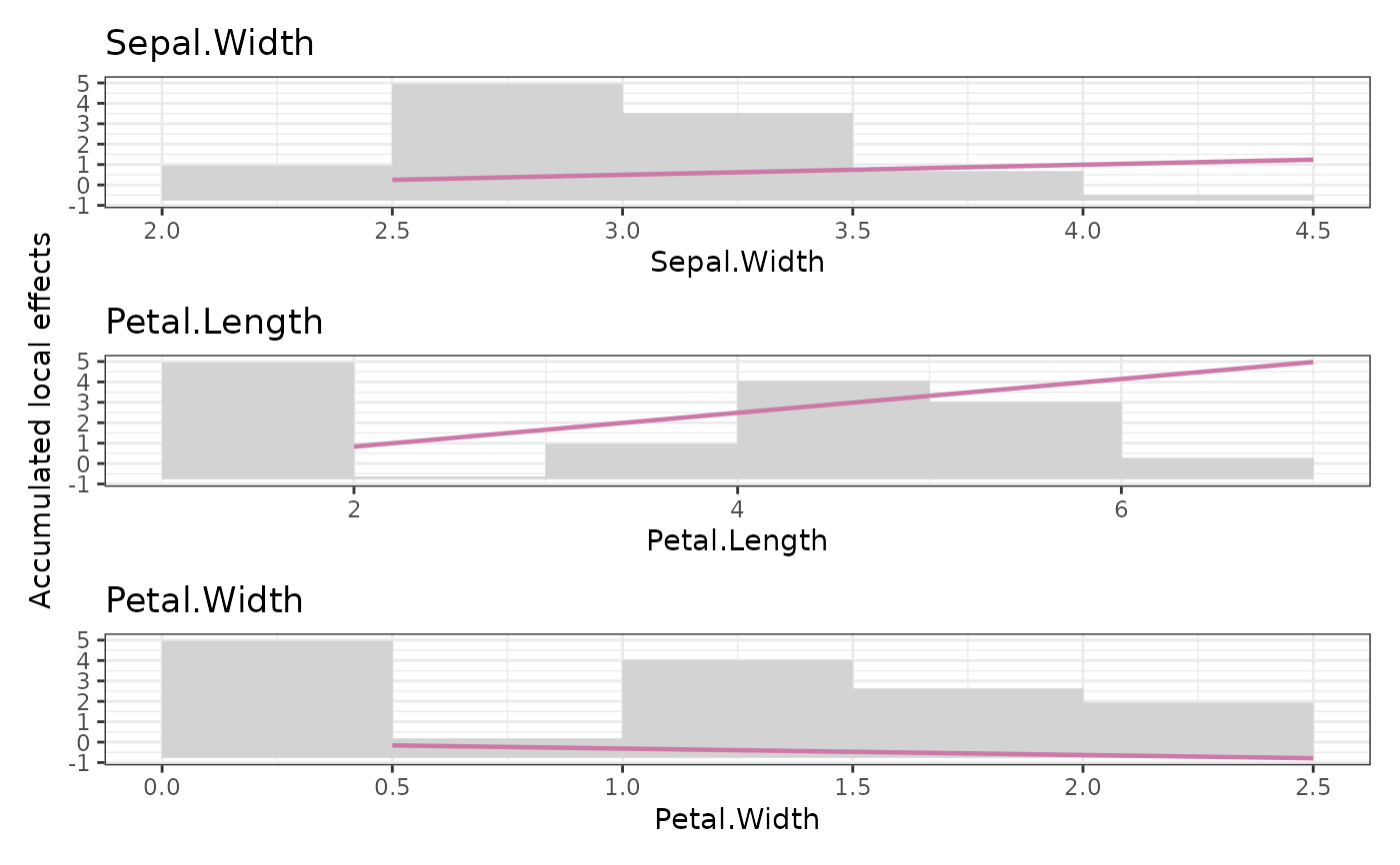
Calculates uncentered ALE for one or multiple continuous features specified by X.
The concept of ALE was introduced in Apley et al. (2020) as an alternative to partial dependence (PD). The Ceteris Paribus clause behind PD is a blessing and a curse at the same time:
Blessing: The interpretation is easy and similar to what we know from linear regression (just averaging out interaction effects).
Curse: The model is applied to very unlikely or even impossible feature combinations, especially with strongly dependent features.
ALE fixes the curse as follows: Per bin, the local effect is calculated as the partial dependence difference between lower and upper bin break, using only observations falling into this bin. This is repeated for all bins, and the values are accumulated.
This implementation closely follows the implementation of Apley et al. (2020).
Notably, we also plot the values at the bin breaks, not at the bin means.
The main difference to Apley is that we use uniform binning, not quantile binning.
For large bins, we sample ale_bin_size observations, a step that is not necessary
with quantile binning. Furthermore, we don't center the values to mean 0.
ale(object, ...)

# Default S3 method
ale(
  object,
  v,
  data,
  pred_fun = stats::predict,
  trafo = NULL,
  which_pred = NULL,
  w = NULL,
  breaks = "Sturges",
  right = TRUE,
  discrete_m = 13L,
  outlier_iqr = 2,
  ale_n = 50000L,
  ale_bin_size = 200L,
  seed = NULL,
  ...
)

# S3 method for class 'ranger'
ale(
  object,
  v,
  data,
  pred_fun = NULL,
  trafo = NULL,
  which_pred = NULL,
  w = NULL,
  breaks = "Sturges",
  right = TRUE,
  discrete_m = 13L,
  outlier_iqr = 2,
  ale_n = 50000L,
  ale_bin_size = 200L,
  seed = NULL,
  ...
)

# S3 method for class 'explainer'
ale(
  object,
  v = colnames(data),
  data = object$data,
  pred_fun = object$predict_function,
  trafo = NULL,
  which_pred = NULL,
  w = object$weights,
  breaks = "Sturges",
  right = TRUE,
  discrete_m = 13L,
  outlier_iqr = 2,
  ale_n = 50000L,
  ale_bin_size = 200L,
  seed = NULL,
  ...
)

# S3 method for class 'H2OModel'
ale(
  object,
  data,
  v = object@parameters$x,
  pred_fun = NULL,
  trafo = NULL,
  which_pred = NULL,
  w = object@parameters$weights_column$column_name,
  breaks = "Sturges",
  right = TRUE,
  discrete_m = 13L,
  outlier_iqr = 2,
  ale_n = 50000L,
  ale_bin_size = 200L,
  seed = NULL,
  ...
)
Arguments
- object
Fitted model.
- ...
Further arguments passed to
pred_fun(), e.g.,type = "response"in aglm()or (typically)prob = TRUEin classification models.- v
Variable names to calculate statistics for.
- data
Matrix or data.frame.
- pred_fun
Prediction function, by default
stats::predict. The function takes three arguments (names irrelevant):object,data, and....- trafo
How should predictions be transformed? A function or
NULL(default). Examples arelog(to switch to link scale) orexp(to switch from link scale to the original scale). Applied afterwhich_pred.- which_pred
If the predictions are multivariate: which column to pick (integer or column name). By default
NULL(picks last column). Applied beforetrafo.- w
Optional vector with case weights. Can also be a column name in
data. Having observations with non-positive weight is equivalent to excluding them.- breaks
An integer, vector, or "Sturges" (the default) used to determine bin breaks of continuous features. Values outside the total bin range are placed in the outmost bins. To allow varying values of
breaksacross features,breakscan be a list of the same length asv, or a named list with breaks for certain variables.- right
Should bins be right-closed? The default is
TRUE. Vectorized overv. Only relevant for continuous features.- discrete_m
Numeric features with up to this number of unique values are treated as discrete and are therefore dropped from the calculations.
- outlier_iqr
If
breaksis an integer or "Sturges", the breaks of a continuous feature are calculated without taking into account feature values outside quartiles +-outlier_iqr* IQR (where <= 9997 values are used to calculate the quartiles). To let the breaks cover the full data range, setoutlier_iqrto 0 orInf. Vectorized overv.- ale_n
Size of the data used for calculating ALE. The default is 50000. For larger
data(andw),ale_nrows are randomly sampled. Each variable specified byvuses the same sample. Set to 0 to omit ALE calculations.- ale_bin_size
Maximal number of observations used per bin for ALE calculations. If there are more observations in a bin,
ale_bin_sizeindices are randomly sampled. The default is 200. Applied after sampling regardingale_n.- seed
Optional integer random seed used for:
ALE: select background data if
n > ale_n, and for bins >ale_bin_size.Calculating breaks: The bin range is determined without values outside quartiles +- 2 IQR using a sample of <= 9997 observations to calculate quartiles.
Value
A list (of class "EffectData") with a data.frame per feature having columns:
bin_mid: Bin mid points. In the plots, the bars are centered around these.bin_width: Absolute width of the bin. In the plots, these equal the bar widths.bin_mean: For continuous features, the (possibly weighted) average feature value within bin. For discrete features equivalent tobin_mid.N: The number of observations within bin.weight: The weight sum within bin. Whenw = NULL, equivalent toN.Different statistics, depending on the function call.
Use single bracket subsetting to select part of the output. Note that each data.frame contains an attribute "discrete" with the information whether the feature is discrete or continuous. This attribute might be lost when you manually modify the data.frames.
Details
The function is a convenience wrapper around feature_effects(), which calls
the barebone implementation .ale() to calculate ALE.
Methods (by class)
ale(default): Default method.ale(ranger): Method for ranger models.ale(explainer): Method for DALEX explainersale(H2OModel): Method for H2O models
References
Apley, Daniel W., and Jingyu Zhu. 2020. Visualizing the Effects of Predictor Variables in Black Box Supervised Learning Models. Journal of the Royal Statistical Society Series B: Statistical Methodology, 82 (4): 1059–1086. doi:10.1111/rssb.12377.

